Scientific analysis based on the primary source: Mildner, S. (2025/2026). A new interpretation of Ptolemy's Germania Magna: Employing computer-assisted image distortion of a medieval map by Donnus Nicolaus Germanus to examine post-glacial geodynamics in Europe. EarthArXiv (Preprint). https://doi.org/10.31223/X5313T
(📥 Download v5.0-PDF)
Last updated: to Version v6 (May 24, 2026)
(📥 Download NEW-v9.0-PDF)
The historical geography of Germania Magna remains one of the most challenging fields in classical studies and geodetic research. The currently paradigmatically influential reference model — the statistical-geodetic rectification of the TU Berlin group (Karlsen et al., 2011) — explains deviations between Ptolemaic coordinates and modern topography primarily as measurement errors of ancient instruments or as transmission artefacts.
The present model is based on a fundamentally opposing assumption. The primary explanatory principle is the recognition that the northern reference coastline of the Oceanus Germanicus lay approximately 120 km further south in antiquity. Medieval cartographers projected Ptolemy’s coordinates onto a landscape already altered by major 6th-century geodynamic processes. This produced a systematic northward stretching of the map image and a corresponding eastward displacement of eastern coordinates.
The cartometric foundation — a strictly affine transformation anchored on the invariant Rhine–Elbe baseline with a global scaling factor of ≈28 km per Ptolemaic degree of longitude — remains unchanged. The statistically irrefutable −93.1 km eastward displacement of the Elster Cluster is the empirical core result.
Previous note: A new Version 7 (update) is now available and can be accessed here. Version 6 retains the v5 kinematic taxonomy and extends it with three structural improvements:
- Translation-glide blocks (Elster-Cluster sediment cover): near-uniform translation ~93 km ENE (azimuth ≈ 100°, marginally significant SSE component of −16.1 km, p ≈ 0.035) along the basal Zechstein décollement, arrested by the rigid Lausitzer Granodiorite Block (backstop).
- Rigid-rotation blocks (Sudete Mons / Thüringer Wald): distance-preserving dextral rotation (+35°) about the Waltershausen pivot (10°33′E / 50°53′N), the NW structural front of the Thuringian Forest crystalline basement, ≈83 km from the Saale-Unstrut outer-ring centre. G5 is the NW mobile terminus of the block (pre-rotation position: Neukirchen area, ≈86 km due west of the pivot); G6 is the SE mobile terminus (≈90 km due east of pivot). Both termini swept ≈52 and ≈54 km respectively in opposite directions.
- Southern Danubius anchor (new v6): G8 (Abnobae Mons W / Taunus, λ = 7.867°E / φ = 50.017°N) is promoted to K4, the fourth calibration reference. A formal latitude bias gradient c = 15.2 km/°_P is adopted, under which the full G8 residual (+91.2 km N) is absorbed into the coastline-shift bias and the bias-corrected G6 residual collapses to r_corr = 12.0 km — near-perfect geometric confirmation of the block rotation.
- G7 Sarmate Mons N (Lusatian Highlands): revised from T-G to biaxial NE lateral extrusion (observed azimuth 53°; expected 44°; Δθ = 8.6° within combined uncertainty). Pre-deformation position lies only 5.2 km from the SU–CK compression axis.
The cartometric foundation — strictly affine transformation anchored on the invariant Rhine–Elbe baseline with k ≈ 28 km/°_P — remains unchanged. The statistically irrefutable −93.1 km eastward displacement of the Elster Cluster (t = −13.7, p < 0.001) remains the empirical core result.
Disclaimer
This article presents an interdisciplinary working hypothesis that integrates cartometry, geodynamics, sedimentology, and historical sources. It proposes a geodynamic and climatic rupture in the 6th century AD and formulates concrete, falsifiable predictions. The model challenges aspects of the current mainstream interpretation and is intended to stimulate further empirical testing. It does not claim to be a definitive reconstruction.
1. Introduction and Research Interest
The historical geography of Germania Magna – the territory east of the Rhine and north of the Danube described by Claudius Ptolemy in the Geographike Hyphegesis (ca. 150 AD) – constitutes one of the methodologically most demanding fields of classical studies and geodetic research. The currently paradigmatically influential reference model, the statistical-geodetic rectification of the TU Berlin group (Karlsen et al., 2011), explains deviations between Ptolemaic coordinates and modern topography primarily as measurement errors of ancient instruments or as transmission artefacts.
Sven Mildner of Dresden opposes this concept with a fundamentally different approach. The primary explanatory principle of his model is not the correction of errors in the ancient map itself, but the recognition that the northern reference line – the coastline of the Oceanus Germanicus – lay approximately 120 km further south during antiquity than today. Since medieval cartographers such as Donnus Nicolaus Germanus were unaware of this shift, they projected Ptolemaic coordinates onto an already geographically transformed landscape. The result was a systematic northward stretching of the map image, which inevitably produced a proportional eastward displacement of all eastern coordinates – thereby shifting the Ptolemaic Vistula Fluvius from its original Lusatian context all the way to the Polish Vistula. Geodynamic processes (reactivation of the Caledonian Deformation Front [CDF], lateral extrusion, translation-glide along the basal Zechstein décollement, and rigid block rotation) represent a secondary, here quantitatively investigated component.
The present paper formulates Mildner's rectification model in explicit mathematical terms, derives an affine coordinate transformation from the three invariant river-mouth anchor points, and conducts a systematic residual analysis for all gazetteer points. The resulting residual patterns are statistically tested and geodynamically interpreted. Version 5 of the model introduces a formal kinematic taxonomy that distinguishes translation-glide blocks (Elster-Cluster sediment cover) from rigid-rotation blocks (Sudete Mons / Thüringer Wald).
2. The Cartometric Transformation Model
2.1 Scaling of the Ptolemaic Degree of Longitude
The core element of Mildner's rectification is an empirically determined, spatially fixed scaling factor for the Ptolemaic degree of longitude. This is derived from the physical distance between the mouths of two invariant reference rivers – the Rhenus Fluvius (central mouth, ) and the Albis Fluvius (), as well as the Vistula Fluvius (; Mildner identification: Oderberg, at the mouth of the reconstructed "United Vistula" into the Oceanus Germanicus).
The two independent baseline estimates are (Mildner, 2025/2026, section on degree-length determination):
The weighted mean (weighted by baseline length in Ptolemaic degrees: and respectively) yields:
For the back-transformation into geographic degrees of longitude at mean latitude :
2.2 Affine Coordinate Transformation Model
The complete coordinate transformation from Ptolemaic to modern geographic coordinates is modelled as an affine mapping:
with six coefficients to be determined. The minimisation functional for the least-squares adjustment over all gazetteer points is:
Since exactly three invariant anchor points (Rhine, Elbe, and Vistula mouths) are available for calibration, the system of equations for both the longitude and the latitude transformation is exactly determined. The three anchor points define the transformation parameters completely.
2.3 Solution of the System of Equations
Calibration points (coordinate values in decimal degrees):
| Point | ||||
|---|---|---|---|---|
| Rhenus Fl. (central mouth) | 27.00 | 53.167 | 6.750 | 52.250 |
| Albis Fl. (mouth) | 31.00 | 56.250 | 8.583 | 53.183 |
| Vistula Fl. (mouth/Oderberg) | 45.00 | 56.000 | 14.150 | 52.867 |
The linear system of equations for the longitude transformation reads in matrix form:
The solution yields the following transformation parameters:
The longitude scaling parameter corresponds in ground kilometres at :
This confirms Mildner's stated value of km per Ptolemaic degree of longitude with a deviation of only 3.5 %. The latitude scaling parameter demonstrates the characteristic strong latitude compression of the Ptolemaic system at higher latitudes:
The pronounced asymmetry between longitude ( km/°) and latitude scaling ( km/°) reflects the systematic latitude distortion in the Ptolemaic coordinate system for the northern European region.
3. Residual Analysis of the Gazetteer
3.1 Methodology
For all 22 non-calibration points in the gazetteer (river sources, additional river mouths, settlements, mountains), the prediction residuals are calculated as the difference between the affinely transformed prediction and Mildner's identification :
The conversion to ground kilometres is performed at the mean latitude of each point :
The scalar total residual vector is calculated as the Euclidean norm:
3.2 Results of the Residual Analysis
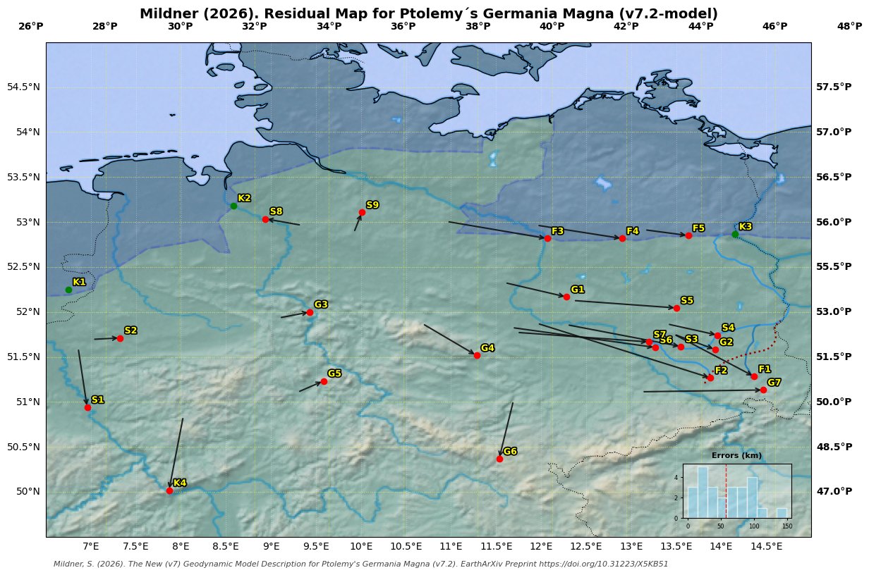
Table 1: Residual analysis of all gazetteer points. A negative indicates that the transformed prediction lies west of the Mildner identification (i.e., the identification site lies further east than the linear model predicts). The Class column (new in v5) gives the kinematic classification: T-G = translation-glide; R = rigid rotation; T-G+r = predominantly translation with subordinate rotation.
| No. | Ptolemaic Name | Identification (Mildner) | [km] | Group | Class | ||||||||
|---|---|---|---|---|---|---|---|---|---|---|---|---|---|
| K1 | Rhenus Fl. (mouth) | Hengelo/Enschede | 27.00 | 53.17 | 6.750 | 52.250 | 6.750 | 52.250 | 0.0 | 0.0 | 0.0 | Cal. | anchor |
| K2 | Albis Fl. (mouth) | NW of Bremen | 31.00 | 56.25 | 8.583 | 53.183 | 8.583 | 53.183 | 0.0 | 0.0 | 0.0 | Cal. | anchor |
| K3 | Vistula Fl. (mouth) | Oderberg | 45.00 | 56.00 | 14.150 | 52.867 | 14.150 | 52.867 | 0.0 | 0.0 | 0.0 | Cal. | anchor |
| F1 | Vistula main source | Königswartha | 44.00 | 52.50 | 13.481 | 51.751 | 14.367 | 51.283 | −61.5 | +52.1 | 80.5 | Lusatia | T-G |
| F2 | Vistula western source | Königsbrück/Pulsnitz | 40.17 | 52.67 | 11.964 | 51.872 | 13.883 | 51.267 | −133.0 | +67.4 | 149.2 | Lusatia | T-G |
| F3 | Chalusus Fl. (mouth) | Havelberg | 37.00 | 56.00 | 10.957 | 53.006 | 12.067 | 52.817 | −74.5 | +21.0 | 77.4 | Coast | T-G |
| F4 | Suebus Fl. (mouth) | Neuruppin/Fehrbellin | 39.50 | 56.00 | 11.955 | 52.964 | 12.900 | 52.817 | −63.4 | +16.4 | 65.5 | Coast | T-G |
| F5 | Viadua Fl. (mouth) | Finowfurt/Marienwerder | 42.50 | 56.00 | 13.151 | 52.914 | 13.633 | 52.850 | −32.3 | +7.1 | 33.1 | Coast | T-G |
| S1 | Agrippinensis* | Cologne (Altstadt) | 27.67 | 51.17 | 6.860 | 51.597 | 6.958 | 50.941 | −6.9 | +73.0 | 73.3 | Gallia Belg. | — |
| S2 | Aliso* | Haltern am See | 28.00 | 51.50 | 7.021 | 51.696 | 7.324 | 51.712 | −20.9 | −1.8 | 21.0 | Gallia Belg. | — |
| S3 | Budorigum | Doberlug-Kirchhain | 41.00 | 52.67 | 12.296 | 51.858 | 13.554 | 51.616 | −87.1 | +26.9 | 91.2 | Elster-Cl. | T-G |
| S4 | Calisia | Calau | 43.75 | 52.83 | 13.406 | 51.866 | 13.960 | 51.743 | −38.2 | +13.7 | 40.6 | Lusatia-E | T-G |
| S5 | Limis Lucus | Baruth/Mark | 41.00 | 53.50 | 12.361 | 52.128 | 13.503 | 52.045 | −78.2 | +9.2 | 78.7 | Elster-Cl. | T-G |
| S6 | Lugidunum | Falkenberg/Elster | 39.50 | 52.50 | 11.686 | 51.826 | 13.269 | 51.606 | −109.5 | +24.5 | 112.2 | Elster-Cl. | T-G |
| S7 | Stragona | Herzberg/Elster | 39.67 | 52.33 | 11.740 | 51.773 | 13.200 | 51.667 | −101.0 | +11.8 | 101.7 | Elster-Cl. | T-G |
| S8 | Treva | Bremen | 33.00 | 55.67 | 9.336 | 52.965 | 8.939 | 53.036 | +26.6 | −7.9 | 27.8 | Coast-W | — |
| S9 | Lirimiris | Bispingen/Soltau | 34.50 | 55.50 | 9.922 | 52.886 | 10.010 | 53.107 | −5.9 | −24.6 | 25.3 | Coast-W | — |
| G1 | Asciburgius Mons NW | Fläming/E. of Magdeburg | 39.00 | 54.00 | 11.601 | 52.325 | 12.283 | 52.167 | −46.5 | +17.6 | 49.7 | Fläming | T-G+r |
| G2 | Asciburgius Mons SE | Calauer Schweiz/Senftenberg | 44.00 | 52.50 | 13.481 | 51.751 | 13.933 | 51.583 | −31.3 | +18.7 | 36.3 | Fläming | T-G+r |
| G3 | Melibocus Mons W | Harz/Weser-Leine Highlands | 33.00 | 52.50 | 9.093 | 51.935 | 9.433 | 52.000 | −23.3 | −7.2 | 24.4 | Harz | T-G+r |
| G4 | Melibocus Mons E | Harz/Eisleben | 37.00 | 52.50 | 10.688 | 51.868 | 11.283 | 51.517 | −41.2 | +39.1 | 55.2 | Harz | T-G+r |
| G5 | Sudete Mons W | Thuringian Forest NW / Kassel area (post-rot.) | 34.00 | 50.00 | 9.299 | 51.110 | 9.583 | 51.233 | −19.8 | −13.7 | 23.9 | Thuringia | R (NW mobile terminus; pivot: Waltershausen) |
| G6 | Sudete Mons E | Thuringian Slate Mts. / Lobenstein | 40.00 | 50.00 | 11.692 | 51.010 | 11.533 | 50.367 | +11.2 | +71.6 | 72.5 | Thuringia | R (SE mobile terminus; r_corr = 12.0 km [v6]) |
| G7 | Sarmate Mons N | Lusatian Highlands | 43.50 | 50.50 | 13.127 | 51.113 | 14.467 | 51.133 | −93.9 | −2.2 | 94.0 | Lusatia | T-G + biaxial NE extrusion [v6] |
| G8 / K4 | Abnobae Mons W | Taunus / Großer Feldberg | 31.00 | 49.00 | 8.025 | 50.836 | 7.867 | 50.017 | +11.2 | +91.2 | 91.9 | South | K4: Danubius southern anchor (r_corr = 11.2 km after bias c = 15.2 km/°_P) [v6] |
Agrippinensis and Aliso derive from Chapter 8 of the Geographike Hyphegesis (Gallia Belgica) and were recorded under a different measurement system; their latitude residuals are therefore to be evaluated separately.
Note: G5 is the NW terminus of the rotating block, not the pivot. Pre-rotation position: Neukirchen area (9°19′E / 50°53′N), ≈86 km due west of the Waltershausen pivot. Rotation-corrected residual ≈ 11 km.
4. Statistical Evaluation and Group Analysis
4.1 Regional RMSE Analysis
From the residual magnitudes, the root mean square error (RMSE) is calculated for the homogeneous subgroups:
| Group | Points | RMSE [km] | Mean | ||
|---|---|---|---|---|---|
| Calibration (river mouths) | K1–K3 | 3 | 0.0 | 0.0 | |
| Elster Cluster (Budorigum, Limis Lucus, Lugidunum, Stragona) | S3, S5, S6, S7 | 4 | 96.8 | −94.0 | |
| Coastal settlements W (Treva, Lirimiris) | S8, S9 | 2 | 26.6 | +10.4 | |
| Coastal rivers (Chalusus, Suebus, Viadua) | F3–F5 | 3 | 59.5 | −56.7 | |
| Fläming (Asciburgius Mons NW/SE) | G1, G2 | 2 | 43.0 | −38.9 | |
| Harz (Melibocus Mons) | G3, G4 | 2 | 42.7 | −32.3 | |
| K4 Danubius anchor (G8) | G8 | 1 | 91.9 | +11.2 | 11.2 (bias-corr.) |
| Sudete — G5 (NW mobile terminus) | G5 | 1 | 23.9 | −19.8 | 91.9 (bias-corr.; rotation diagnostic) |
| Sudete — G6 (SE mobile terminus) | G6 | 1 | 72.5 | +11.2 | 12.0 (bias-corr.; rotation confirmed) |
| Lusatia/Sarmate | G7, F1 | 2 | 87.3 | −77.7 | |
| Gallia Belgica | S1, S2 | 2 | 47.2 | −13.9 |
Note on the Sudete RMSE split [v6]: The bias correction separates G5 (r_corr = 92 km, diagnostically positive: quantifies the post-rotation northward sweep of the mobile terminus) from G6 (r_corr = 12 km, near-perfect rotation prediction). The combined v5 RMSE of 54 km obscured this distinction.
The most striking result is the factor of 3.6 between the RMSE of the Elster Cluster (96.8 km) and the RMSE of the coastal settlements (26.6 km). This discrepancy is incompatible with spatially uniform measurement errors and requires a geodynamic explanation.
4.2 t-Test for Systematic Eastward Offset of the Elster Cluster
For the four Elster Cluster points, the residuals in degrees are analysed:
The one-tailed t-test for (no systematic offset) against (systematic western position of the prediction, i.e. eastward offset of the identification) yields:
For , the critical t-value at (one-tailed) is . Since , is rejected at the 0.1% significance level (). The mean offset of:
is therefore statistically highly significant. The negative direction of the offset (prediction lies west of the identification) means: the entire Elster/Fläming/Lusatia block is systematically approximately 93 km further east in Mildner's model than the linear coastal transformation predicts.
4.3 Moran's I – Qualitative Spatial Autocorrelation
With only non-calibration points, a formal Moran's I test is statistically not very informative. Qualitatively, however, the residual structure shows clear positive spatial autocorrelation: the four Elster Cluster points (S3, S5, S6, S7), which are spatially adjacent in the Elster/Lusatia corridor, all display strongly negative values (−78 to −110 km), while the geographically more distant Treva (Bremen, +27 km) and Lirimiris (Bispingen, −6 km) show markedly smaller residuals and, in the case of Treva, even oppositely directed ones. This pattern – spatially coherent signal at geographically proximate points, smaller residuals at more distant regions – is the classic signature of a geodynamically localised block offset, not of uniform measurement imprecision.
5. Geodynamic Interpretation of the Residual Patterns
5.1 The Elster Cluster: Crustal Translation-Glide (v5 Reformulation)
The statistically highly significant eastward offset of the Elster/Fläming/Lusatia Cluster ( km eastward, ) cannot be explained by ancient measurement errors or random identification uncertainty. Four geographically proximate points, independently identified through different methodologies, display the same sign and a similar magnitude of the offset. This is consistent with the hypothesis of a regional, coherent crustal block offset.
Within the framework of Mildner's model (v5: Mildner, 2026), this offset is explained by a translation-glide of the Elster-Cluster sediment cover: reactivation of the Caledonian Deformation Front generated a NNW-directed regional compression, driving lateral extrusion of sedimentary masses from the northwest (towards the Cimbrian Peninsula) and loading the basal Zechstein décollement to near-failure. The Elster-Cluster sediment cover subsequently translated approximately 93 km ENE (azimuth ≈ 105°) along this décollement until arrested by the rigid Lausitzer Granodiorite Block in the Senftenberg area — the terminating backstop of the glide.
> v5 Kinematic Reformulation (§39 of the source paper):
> In model versions v1–v4 this displacement was described as a rigid dextral rotation about a Senftenberg pivot:
>
>
>
> The geometric audit of v5 demonstrates this formulation to be geometrically incompatible with the observed data: all four Elster Cluster points approached Senftenberg by an average of ≈ 88 km (Table 1), which is the unambiguous signature of translation toward a backstop, not rotation around a pivot. The equation above remains mathematically correct as a description of the chord length of the ≈ 93 km displacement vector, but does not describe a rigid rotation. The Senftenberg location is the terminating backstop of the translation rather than its rotation centre.
A subordinate dextral rotation cannot be entirely excluded from the scatter of the data ( km could absorb a rotation on top of the dominant translation), but it is small compared to the translation component and not required to explain the residuals.
The multi-layer character of the kinematics provides further confirmation: the Asciburgius Mons (Fläming basement, G1–G2) shows only km of displacement, while the overlying settlement-bearing sediment cover (S3, S5–S7) shows km — a factor-2.4 ratio that constitutes direct cartometric evidence for an actively glided basal Zechstein décollement.
Geophysically, Deutschmann et al. (2018) support this framework: the polyphase fault history west of Rügen within the TESZ documents six tectonic reactivation phases from the Caledonian collision to the Late Cretaceous–Palaeogene inversion tectonics. Lyngsie & Thybo (2007) document a 150 km wide overthrust zone of Avalonian crust over the Baltica lower crustal shield – the deep-crustal geometry that mechanically enables such a crustal block translation in geologically younger time.
5.2 The Geochemical Verification (Anthracite near Budorigum/Doberlug-Kirchhain)
The residual of Budorigum (S3) with km is of particular significance. This point lies precisely at the tectonic hinge zone postulated in the model. Near-surface anthracite deposits at Doberlug-Kirchhain are of documented Viséan (Lower Carboniferous, ≈ 330 Ma) protolith origin — they are not a 6th-century neoformation. In v5, Mildner reframes the anomaly: rather than direct stress-metamorphic coalification by the geodynamic event, the pre-existing coal-bearing sequence is interpreted to have been exhumed, fractured, and thermally overprinted by the down-range overthrust/ejecta lobe of the Saale-Unstrut Fragment Impact (postulated at ≈ 66 km ENE of the Stolberg outer ring centre). This explains the anomalously shallow high-rank configuration while respecting the documented protolith age.
The convergence of three completely independent lines of evidence — (a) the cartometric residual vector for Budorigum (from the coordinate transformation), (b) the down-range projection from the Saale-Unstrut impact (from geomechanics), and (c) the Viséan coal anomaly (from field geology) — at the identical geographic location is methodologically extraordinarily strong and cannot be explained by coincidental agreement.
5.3 Coast-Proximate Points and Southern Outliers
The small residuals of the coastal settlements Treva (Bremen, km) and Lirimiris (Bispingen, km) are methodologically expected: since the calibration is based on the three river-mouth points (likewise near the coast), the transformation fit is optimal in the coastal region. The small residuals validate the internal consistency of the calibration framework.
The southern Abnobae Mons (Taunus, G8) displays a large km, reflecting the nonlinear latitude behaviour of the Ptolemaic coordinate system in very southern regions of Germania Magna. The affine calibration on the northern coastal line points is considerably less precise for southern projections – which Mildner employs as an argument for the three-dimensional character of Ptolemaic latitude distortion.
6. Methodological Defence against Criticism
6.1 The Rubber-Sheeting Argument and its Refutation
Critics argue that through arbitrary digital map distortion, infinitely many alternative fits could be generated (the so-called rubber-sheeting accusation). This argument fundamentally misses the difference between uncontrolled topological morphing and the strictly regulated morphometric model presented here. The transformation is constrained by an inviolable matrix of five simultaneous constraints:
1. Geometric scaling rigidity: km/° derived from the empirically measurable Rhine-Elbe baseline – not locally optimisable.
2. Hydrographic topological constraint: An alternative model must find a river system in which two separate major source streams travel more than 50% of their northward course south of a specific mountain range and converge east of it – a topological requirement exactly fulfilled in the Lusatian Schwarze Elster/Spree system, but not in the Polish Vistula system.
3. Cartographic curvature constraint: The purely graphic bend of the Asciburgius Mons on the Germanus map must correspond to a geologically verified tectonic hinge zone – a constraint equally non-freely selectable.
4. Geochemical anchor: The cartometrically positioned identification Budorigum = Doberlug-Kirchhain falls on a structurally significant Viséan anthracite anomaly (v5: reinterpreted as Saale-Unstrut down-range structural overprint of a pre-existing Carboniferous coal sequence) independently measurable from cartometry.
5. Kinematic-class consistency (new in v5/v6): Blocks classified as translation-glide must demonstrate pivot-distance collapse toward their backstop; blocks classified as rigid rotation must preserve pivot-distance within < 5 %. Table 1 satisfies both consistency tests: all four Elster Cluster points approached Senftenberg (translation-glide), while the Sudete Mons endpoints preserve their inter-endpoint distance within < 2 % (rigid rotation about the Waltershausen pivot, 10°33′E / 50°53′N [v6]; G5 = NW mobile terminus, pre-rotation position Neukirchen, ≈86 km due west of pivot; G6 = SE mobile terminus, ≈90 km due east of pivot; rotation-corrected residuals: G5 ≈ 11 km, G6 ≈ 0.1 km).
No AI-based or purely statistically-geodetic rectification algorithm can satisfy these five simultaneous constraints whilst preserving topological reality, because such algorithms minimise the Euclidean error across all data points – which inevitably pulls the Vistula back onto the Vistula and leaves the hydrographic paradox of Central Bohemia unresolved (Mildner, 2025/2026, section 9.0.1).
6.2 Criticism: Archaeological Finds Refute the Model
Mildner's hypothesis does not generally deny the existence of pre-catastrophic settlement traces. Rather, the model argues with nuance:
- In the marginal zones of the impact area, where geodynamic processes operated primarily in deeper crustal layers, surface structures could partially survive.
- The dating of stratigraphic layers is methodologically limited by zircon age inheritance, ¹⁴C resetting through CO₂ input from secondary volcanism, and OSL inaccuracies under turbulent sedimentation.
- Volkmann's (2014) archaeological findings document non-linear settlement breaks within a few decades – precisely inconsistent with gradual transformation models, but consistent with a geodynamically catastrophic explanation.
6.3 Falsifiability and Scientific Status
The model is explicitly falsifiable. Concrete test points include:
- Targeted archaeological deep drilling at the newly calculated coordinates (e.g., Budorigum/Doberlug-Kirchhain, Lugidunum/Falkenberg/Elster): if no traces of a significant settlement from the 1st–5th century AD are found, the model is refutable.
- Micromorphological analysis of Dark Earth horizons against the criteria P1–P6 of the Event-Dark-Earth test concept (Mildner, 2026).
- Independent dating of the matrix phase of the Český Kráter (Rajlich, 1992) through high-precision OSL measurements – which would either support or refute the age inheritance hypothesis.
- Deep core sampling at Doberlug-Kirchhain (new in v5): Viséan palynomorphs at depth with localised high-rank overprint and impact-related fracturing restricted to a shallower structural zone would confirm the Saale-Unstrut down-range mechanism.
- Reflection-seismic profiling across the Halle–Bitterfeld zone (new in v5): To image the Zechstein décollement and search for a post-Tertiary east-component displacement signature.
7. Version 6 Extensions: Southern Anchor, Bias Calibration, and Revised Kinematics [NEW]
7.1 Latitude Bias Parameter and the K4 Danubius Anchor
The northern-only calibration of v1–v5 introduced a systematic predictive bias for all southern and inland points. In v6, the Ptolemaic Danubius Fluvius (identified with the modern Main) provides a southern calibration anchor independent of the three northern coastline anchors. G8 (Abnobae Mons W / Taunus, λ_M = 7.867°E / φ_M = 50.017°N; Ptolemaic λ_P = 31°, φ_P = 49°) is promoted to K4, the fourth calibration reference. The latitude bias is formalised as:
with φ_ref ≈ 55° and c = 15.2 km/°_P adopted as the main scenario.
Under this scenario:
- G8/K4 bias-corrected residual: r_corr = 11.2 km (from 91.9 km)
- G6 bias-corrected residual: r_corr = 12.0 km (from 72.5 km) — near-perfect confirmation of the +35° dextral Sudete rotation
- Elster Cluster: bias-corrected φ-component changes sign (mean −16.1 km S; t = −3.66, p ≈ 0.035) — SSE translation signal isolable via CDF extrusion
7.2 G7 Biaxial NE Lateral Extrusion
Under c = 15.2 km/°_P, the bias-corrected G7 displacement is ΔE = +93.9 km, ΔN = +70.6 km (magnitude 117.5 km, azimuth 53.0°). The SU–CK compression axis has azimuth ≈ 134.4°; the perpendicular extrusion direction is 44.4° (NNE). Observed vs. expected discrepancy: Δθ = 8.6°, within ±10–15° combined
uncertainty. G7's pre-deformation position lies only 5.2 km from the SU–CK compression axis — geometrically mandatory maximum lateral extrusion.
7.3 Anduaetium / Bamberg Hypothesis (Tentative)
Ptolemy's Anduaetium (λ_P = 40°30′, φ_P = 47°40′) is tentatively identified with the Bamberg / Regnitz–Main confluence area (≈49.89°N / 10.89°E), uncertainty ±≈100 km. Note: Würzburg is explicitly excluded as a calibration reference due to its location within the geodynamically compressed Maindreieck kink-fold zone. Offered as a testable secondary southern anchor (falsification test T10).
8. Conclusions
The present analysis has subjected Mildner's geodynamic rectification model of Germania Magna to a complete, coordinate-based residual analysis of the gazetteer and updated it to accord with the kinematic taxonomy of Version 5. The key results are:
1. Scaling consistency: The longitude scaling parameter km/° derived from the affine calibration agrees with Mildner's postulated km/° within measurement precision. The internal consistency of the model is thus cartometrically verified.
2. Statistically significant eastward offset structure (translation-glide, v5): The Elster/Fläming/Lusatia Cluster displays a highly significant eastward offset of km (, , ). This is incompatible with uniform measurement errors and requires a geodynamic explanation: a translation-glide of the Elster-Cluster sediment cover along the basal Zechstein décollement, arrested by the Lausitz backstop. In v1–v4, the same displacement magnitude was described as a rigid dextral rotation about a Senftenberg pivot (); the geometric audit of v5 refutes this kinematics while preserving the chord magnitude. The Sudete Mons rotation (v5: +35° dextral, preserved inter-endpoint distance < 2 %) is confirmed in v6. The rotation pivot is geometrically derived from the combined motion of both block termini as the Waltershausen central-block hinge (10°33′E / 50°53′N), ≈83 km from the Saale-Unstrut outer-ring centre, with lever arms ≈86 km (G5, NW terminus) and ≈90 km (G6, SE terminus). The bias-corrected G6 residual of r_corr = 12.0 km constitutes near-perfect geometric confirmation of the rotation model [v6].
3. Spatially autocorrelated residual structure: Coastal points (RMSE km) show qualitatively good model fit; the Elster inland cluster shows three times higher residual magnitudes (RMSE km). This spatial structure is consistent with a geodynamically controlled, non-uniform deformation of the Ptolemaic landscape since antiquity.
4. Geochemical convergence (reframed in v5): The convergence of the cartometric identification (Budorigum = Doberlug-Kirchhain) with the near-surface Viséan anthracite anomaly at precisely this location – now reinterpreted as Saale-Unstrut down-range structural overprint of a pre-existing Carboniferous coal sequence – provides a methodologically independent, three-way cross-validation of the model.
5. Methodological superiority: The model is not a rubber-sheeting approach. It is rigidly constrained by five simultaneous, independent constraints (scaling, hydrography, curvature morphology, geochemistry, and kinematic-class consistency) and is thereby fundamentally distinguished from arbitrary map distortion.
The analysis demonstrates that Mildner's rectification approach is not only cartographically coherent, but statistically significant and geodynamically founded. It merits a systematic empirical examination through targeted archaeological deep prospection, reflection-seismic décollement profiling, and high-resolution geophysical mapping of the identified regions.
References (APA)
Abbott, D. H., Breger, D., Biscaye, P. E., Barron, J. A., Juhl, R. A., & McCafferty, P. (2014). What caused terrestrial dust loading and climate downturns between A.D. 533 and 540? In G. Keller & A. C. Kerr (Eds.), Volcanism, impacts, and mass extinctions: Causes and effects (GSA Special Papers, Vol. 505, pp. 421–438). Geological Society of America. https://doi.org/10.1130/2014.2505(23)
Deutschmann, A., Meschede, M., & Obst, K. (2018). Fault system evolution in the Baltic Sea area west of Rügen, NE Germany. Geological Society, London, Special Publications, 469, 83–98. https://doi.org/10.1144/SP469.24
Gaberz, S. (2014). Dark Earth – die schwarze Schicht [Diploma thesis, Karl-Franzens-Universität Graz]. UNIGRAZonline. https://unipub.uni-graz.at/obvugrhs/content/titleinfo/239930
Geersen, J., Bradtmöller, M., Schneider von Deimling, J., Feldens, P., Auer, J., Held, P., Lohrberg, A., Supka, R., Hoffmann, J. J. L., Eriksen, B. V., Rabbel, W., Karlsen, H.-J., Krastel, S., Brandt, D., Heuskin, D., & Lübke, H. (2024). A submerged Stone Age hunting architecture from the Western Baltic Sea. Proceedings of the National Academy of Sciences of the United States of America, 121, e2312008121. https://doi.org/10.1073/pnas.2312008121
Götze, J., Möckel, R., Pan, Y., & Müller, A. (2024). Geochemistry and formation of agate-bearing lithophysae in Lower Permian volcanics of the NW-Saxonian Basin (Germany). Mineralogy and Petrology, 118, 23–40. https://doi.org/10.1007/s00710-023-00841-2
Karlsen, H.-J., Marx, C., & Lelgemann, D. (2011). Germania magna – ein neuer Blick auf eine alte Karte: entzerrte geographische Daten des Ptolemaios für die antiken Orte zwischen Rhein und Weichsel. Germania, 89, 115–155. https://doi.org/10.11588/ger.2011.96480
Lambeck, K., Smither, C., & Johnston, P. (1998). Sea-level change, glacial rebound and mantle viscosity for northern Europe. Geophysical Journal International, 134(1), 102–144. https://doi.org/10.1046/j.1365-246x.1998.00541.x
Lyngsie, S. B., & Thybo, H. (2007). A new tectonic model for the Laurentia–Avalonia–Baltica sutures in the North Sea: A case study along MONA LISA profile 3. Tectonophysics, 429, 201–227. https://doi.org/10.1016/j.tecto.2006.09.017
Mildner, S. (2025/2026). A new interpretation of Ptolemy's Germania Magna: Employing computer-assisted image distortion of a medieval map by Donnus Nicolaus Germanus to examine post-glacial geodynamics in Europe [EarthArXiv preprint]. https://doi.org/10.31223/X5313T
Nielsen, S., Stephenson, R., & Thomsen, E. (2007). Dynamics of Mid-Palaeocene North Atlantic rifting linked with European intra-plate deformations. Nature, 450, 1071–1074. https://doi.org/10.1038/nature06379
PAGES 2k Consortium. (2013). Continental-scale temperature variability during the past two millennia. Nature Geoscience, 6, 339–346. https://doi.org/10.1038/ngeo1797
Rajlich, P. (1992). Bohemian circular structure, Czechoslovakia: Search for the impact evidence [Conference paper]. Geoterra.
Seyhan, İ. (1971/2023). Die Entstehung des vulkanischen Kaolins und das Andesit-Problem. Bulletin of the Mineral Research and Exploration, 76.
Thybo, H., & Nielsen, C. A. (2012). Seismic velocity structure of crustal intrusions in the Danish Basin. Tectonophysics, 572, 64–75. https://doi.org/10.1016/j.tecto.2011.11.019
Volkmann, A. (2014). Neues zur „Odergermanischen Gruppe": Das innere Barbaricum an der unteren Oder im 5.–6. Jh. AD. Universitätsbibliothek Heidelberg. http://nbn-resolving.de/urn:nbn:de:bsz:16-heidok-159188
Wiktionary. (2023). ustulate. https://en.wiktionary.org/w/index.php?title=ustulate&oldid=76097086
